A GTFS feed is a standardised format used by public transportation agencies to provide schedule, route, and geographic data, enabling developers to create applications that offer transit information and services to the public. If you're a transport planner, they can often be the bane of your existence…
As a transport planner, when working with a General Transit Feed Specification (GTFS) feed, understanding what constitutes an ‘average week’ is useful for gaining insights into the typical service patterns and usage trends.
By ‘average week’, we mean the date range that best represents the overall service level and activity within the transit system, serving as a benchmark for comparison and analysis.
Determining the average week is not a one-size-fits-all task. It involves careful consideration of various factors, including the distribution of trip counts, presence of service outliers and the inherent variations in transit usage across different weeks. This layer of complexity is often influenced by factors such as holidays, events, and seasonal fluctuations.
At Podaris, we spend a lot of time building clever ways to process, simplify, and analyse GTFS feeds to help support the transport planners that use the plaform. In this article, we'll explore why automatically finding the “average” week can be so challenging, and the types of things you might want to consider.
To calculate the average week, we can use various statistical methods that each address different aspects of the data distribution. These methods help identify weeks that align closely with the typical service levels. The choice of method depends on the characteristics of the feed, sensitivity to outliers and the goals of the analysis.
Contrasting Methods for Calculating the Average Week in a GTFS Feed
The statistical methods we will contrast include:
Average by Z-Score
- Method: The average week is determined based on the z-score of the weekly trip counts, with the one closest to zero (i.e. the mean) being considered the average
- Advantages:
- Accounts for data variability by measuring standard deviations (the distance) from the mean
- Disadvantages:
- Assumes a normal distribution, which might not hold for all GTFS feeds
- Sensitive to outliers, potentially leading to inaccurate results
- Edge Cases/Considerations:
- Highly skewed distributions can lead to incorrect average week identification
Average by Median
- Method: The median week is chosen as the average week, representing the middle value when data is sorted
- Advantages:
- Unaffected by outliers, providing a representative typical week in trip counts
- Disadvantages:
- Ignores distribution shape, potentially missing nuances
- Edge Cases/Considerations:
- Effective for feeds with a skewed data distributions or when outliers are common
Average by Mode
- Method: The average week is determined by the week with a trip count that occurs the most often in the dataset
- Advantages:
- Helps highlight the most common service patterns that passengers are likely to encounter by considering peak levels
- Like median, the mode is robust to outliers
- Disadvantages:
- Sensitive to small changes in data, adding or removing a single value can lead to a different mode
- No consideration for the variability within the dataset
- Edge Cases/Considerations
- If the data for certain days of the week is sparse or missing, calculating the mode might not accurately represent the true patterns
Choosing the Right Method
Based on the advantages and disadvantages we can summarise that we should:
- Use the average by z-score for normally distributed data with potential anomalies
- Use the median or modal average when seeking robustness against outliers

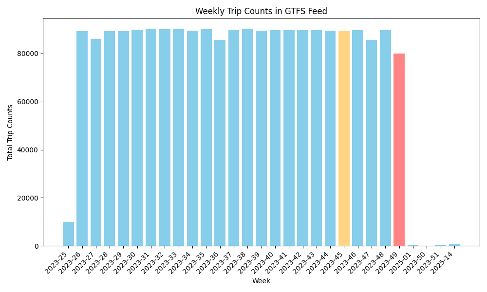
In the above example, we see the data from a GTFS feed with trip counts on the Y-axis, and the year and week number that the trips occurred on the X-axis. Although mostly uniform, we can see that on the extremeties of the chart service levels drop dramatically, likely due to public holidays observered at the beginning/end of the year. Week 2023-45 was identified as the average week using the median average while 2023-49 being identified by z-score.
With latter week having a trip count that is less than ~80% of the others, we can assume that this is not actually representative of the average.
As mentioned before one of the key disadvantages of z-score is its sensitivity to outliers. This is due to the fact that the scores assigned to each week are determined by their distance to the mean, a metric which itself is sensitive to outliers.
To get a better average using the z-score average (or any mean-based average method) we can ‘trim’ a certain percentage of values from either side of the dataset.
The idea being that in doing so, the method will provide a more robust estimate of central tendency that is less influenced by outliers.
In the case of the feed above, a more accurate average is only achieved with a trim level of 30%, i.e. we remove 4 months from either end. In this case, the z-score average given is week 2023-47, which seems to be more representative of overall service levels.

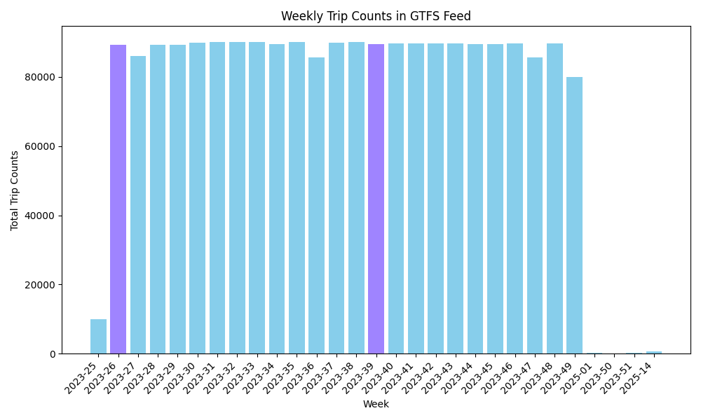
The two weeks defined as ‘average’ by using mode were 2023-26 and 2023-39.
We can see that by simply considering the weeks with trip counts that occur the most, the average weeks identified look to be more representative of service as a whole. This works for feeds that model services that have trip counts that are generally consistent but would fall short of accuracy when considering a transit system that exhibits more erratic behaviour over the course of the year.
To conclude, when working with GTFS data, the dynamic nature of transportation systems can lead to difficulties that require extra consideration in order to get right.
This article was written by Daniel Famiyeh, a dedicated full stack software developer who at Podaris has made significant enhancments to the GTFS tools within the platform.
Daniel's journey into software commenced within the captivating realm of the Sony PSP homebrew scene at the age of 11. This initial spark ignited a passion for Python scripting and experimenting with JavaScript to create 2D games using the Canvas API. Daniel's early engagement with web development, crafting Tumblr themes for personal and friends’ use, laid the groundwork for a future reconnection with this dynamic field.
